Runs the app in the development mode.
Open http://localhost:3000 to view it in the browser.
The page will reload if you make edits.
You will also see any lint errors in the console.
npm test
Launches the test runner in the interactive watch mode.
See the section about running tests for more information.
npm run build
Builds the app for production to the build folder.
It correctly bundles React in production mode and optimizes the build for the best performance.
The build is minified and the filenames include the hashes.
Your app is ready to be deployed!
See the section about deployment for more information.
npm run eject
Note: this is a one-way operation. Once you eject, you can’t go back!
If you aren’t satisfied with the build tool and configuration choices, you can eject at any time. This command will remove the single build dependency from your project.
Instead, it will copy all the configuration files and the transitive dependencies (webpack, Babel, ESLint, etc) right into your project so you have full control over them. All of the commands except eject will still work, but they will point to the copied scripts so you can tweak them. At this point you’re on your own.
You don’t have to ever use eject. The curated feature set is suitable for small and middle deployments, and you shouldn’t feel obligated to use this feature. However we understand that this tool wouldn’t be useful if you couldn’t customize it when you are ready for it.
This repository contains code for sparse scene flow estimation using stereo cameras, proposed by P. Lenz etal.: Sparse Scene Flow Segmentation for Moving Object Detection in
Urban Environments, Intelligent Vehicles Symposium (IV), 2011.
This method can be used as a component in your
visual object tracking / 3D reconstruction / SLAM applications
as an alternative to dense (and typically expensive to compute) scene flow methods.
Note: The repository contains scene flow estimator only, there is no implementation for scene flow clustering or object tracking provided in this repository.
If you want to know what is the difference between scene and optical flow,
see this quora thread.
For optimal performance, run the sf-estimator in release mode.
UPDATE (Jan’20): I added bindings for python and removed most of the “old” exmaple code in order to shrink the dependencies to the minimum. See the python example.
If you find this code useful in your research, you should cite:
@inproceedings{Lenz2011IV,
  author = {Philip Lenz and Julius Ziegler and Andreas Geiger and Martin Roser},
  title = {Sparse Scene Flow Segmentation for Moving Object Detection in Urban Environments},
  booktitle = {Intelligent Vehicles Symposium (IV)},
  year = {2011}
}
Copyright (c) 2017 Aljosa Osep
Permission is hereby granted, free of charge, to any person obtaining a copy of this software and associated documentation files (the “Software”), to deal in the Software without restriction, including without limitation the rights to use, copy, modify, merge, publish, distribute, sublicense, and/or sell copies of the Software, and to permit persons to whom the Software is furnished to do so, subject to the following conditions:
The above copyright notice and this permission notice shall be included in all copies or substantial portions of the Software.
THE SOFTWARE IS PROVIDED “AS IS”, WITHOUT WARRANTY OF ANY KIND, EXPRESS OR IMPLIED, INCLUDING BUT NOT LIMITED TO THE WARRANTIES OF MERCHANTABILITY, FITNESS FOR A PARTICULAR PURPOSE AND NONINFRINGEMENT. IN NO EVENT SHALL THE AUTHORS OR COPYRIGHT HOLDERS BE LIABLE FOR ANY CLAIM, DAMAGES OR OTHER LIABILITY, WHETHER IN AN ACTION OF CONTRACT, TORT OR OTHERWISE, ARISING FROM, OUT OF OR IN CONNECTION WITH THE SOFTWARE OR THE USE OR OTHER DEALINGS IN THE SOFTWARE.
You will need to enable 3-legged OAuth in the Twitter Developers Dashboard. Make sure to also add your callback URL.
Add provider event listener
Laravel 11+
In Laravel 11, the default EventServiceProvider provider was removed. Instead, add the listener using the listen method on the Event facade, in your AppServiceProviderboot method.
Note: You do not need to add anything for the built-in socialite providers unless you override them with your own providers.
JBoot is a utility for scheduling and executing system reboots with optional tasks using custom logic. JBoot allows you to schedule reboots for computers, customize actions to perform on reboot, and handle various use cases that involve system restarts.
JBoot is designed to provide a simple and flexible way to schedule system reboots. It allows you to specify the desired reboot time, and optional tasks to run on reboot. JBoot also offers enhanced control over system restarts.
Traditional reboot methods are often limited in their capabilities. JBoot aims to address these limitations by providing an intuitive interface to manage and execute reboots while allowing you to define custom behavior based on your requirements.
Maven
To use JBoot in your Maven project add this dependency to the dependencies section of the pom.xml file within your project.
This section provides an example of scheduling system reboots for a particular time using the RebootScheduler classes scheduleRebootAt(rebootDate) method.
publicstaticvoidmain(String[] args) {
RebootSchedulerscheduler = newRebootScheduler();
DaterebootDate = /* Specify a desired reboot date and time */;
scheduler.scheduleRebootAt(rebootDate);
}
Scheduled Reboot With Restart Customization
This section illustrates how to use the scheduleProgrammedReboot() method to schedule a system reboot at a specific date and time, along with a custom task to run on reboot.
publicstaticvoidmain(String[] args) {
RebootSchedulerscheduler = newRebootScheduler();
DaterebootDate = /* Specify a desired reboot date and time */;
StringcustomTask = /* Define a custom task to run on reboot (e.g. path/to/App.exe)*/;
scheduler.scheduleProgrammedReboot(rebootDate, customTask);
}
Contributions
Contributions to JBoot are welcome! If you’d like to contribute, please follow these steps:
Fork the repository and create a new branch for your feature or bug fix.
Make your changes and submit a pull request.
Provide a clear description of your changes and their purpose.
Kademlia is an ingenious distributed hash-table (DHT) protocol that makes use of the XOR metric to measure “distance” between peers. Keys and values are given to the K-closest peers to the hash (256-bits in our case) of the given key. Because of the XOR metric, we can find the K-closest peers in time proportional to the log of the size of the network. That means in a network with a million peers, it might only take about 20 steps to find those responsible for a given key.
This is a work in-progress. I am writing it in C because I like the challenge.
External Dependencies
The two external dependencies that cannot be resolved via the git submodule command below are libuv and openssl. The first is a cross-platform library used for asynchronous I/O operations. The second is a library used for the SHA256 hash function.
Create your own features using custom data and pre-trained models.
Utilizing google colab notebook we take an existing model and re-train to detect our own custom object.
Introduction
Creating deep learning models from scratch can be time consuming and not the best use of your time. We are fortunate to have many pre-trained models available that we can use as a starting point for our own applications. We can use transfer learning to re-train only a small portion that we need in order to develop our feature or solve our problem.
For this project we will be re-training a base Model SSD-mobilenet-v1 pre-trained on the PASCAL
VOC dataset for object detection. We will download data from Google Open Images to retrain the
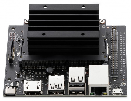
model to detect a custom object class (vehicle license plate). We will then convert and deploy the model
onto an Nvidia Jetson Nano.
Download dataset for training
Our base model can detect 20 objects out of the box but we want to re-train it to detect license plates.
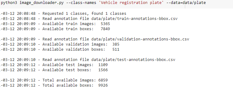
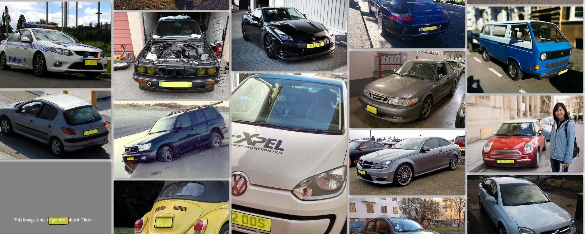
We will be using Google Open Images to download our dataset. We have a choice of 600 different
classes but we will be using ‘Vehicle registration plate’ for our model. Using the website’s provided
script, we end up downloading 6800 images conveniently split up into test/train/validation. This
process can be done with any number of classes but we will be using one class for our example.
The images themselves vary quite a bit in terms of viewing depth/angles and license plate types. We
will be trying to detect USA license plates but our dataset includes plates from all over the world.
Another big limitation of this dataset is its high variance in viewing angles, distances, cars and plate types.
Unfortunately, many of the highly curated datasets related to this particular object class are
proprietary and hard to find.
Re-training existing model
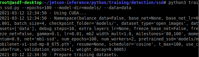
For this project we first re-trained on the Jetson Nano 2gb using the provided Jetson Utitlities script
with 100 epochs.
The 2Gb Nano is not very powerful for training and as a result takes almost 5 days to train. A faster
way to do this is by using Google Colab or your own higher powered GPU. We trained 100 epochs in
6.7 Hours using Google Colab on an Nvidia T4. The average time per epoch on the Nano was 86.
mins while Google Colab took 4 mins per epoch.
At the end of our training we achieved a loss of 2.78.
Model Evaluation
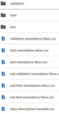
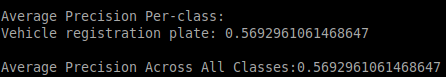
The next step is to evaluate our model against some test data. Fortunately, during our initial
download of our Open Images dataset we created a test folder we can use to evaluate. The test
folder has 1109 Images. Running our evaluation script, we achieve a mAP of .569. Getting more than half recognition is ok performance but again the test set pictures are quite variable. Some pre-trained license plate detection models can have mAP of over 90%.
The next step is to convert this model and deploy it to our Jetson Nano.
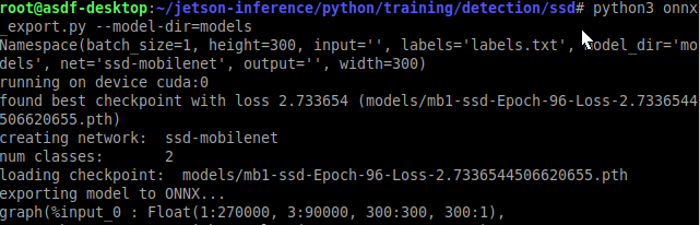
Export and Deploy to Edge Device’
After re-training our model we need to convert it to an .onnx file to load onto the Jetson Nano.
ONNX is an open model format that supports many of the popular ML frameworks, including PyTorch, TensorFlow, TensorRT, and others, so it simplifies transferring models between tools.
We can use the onnx_export.py script provided by jetson utilities. Then with TensorRT (pre-loaded onto the nano) we can optimize the model for deployment on the Jetson Nano.
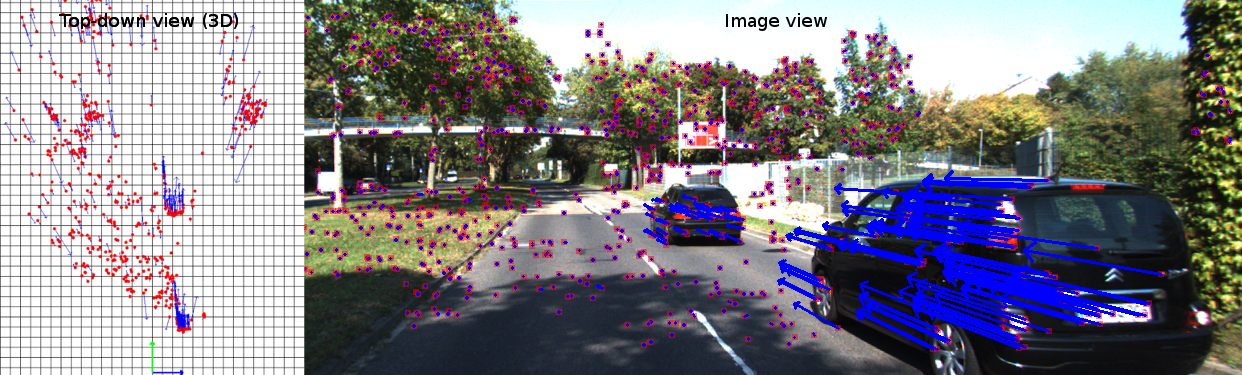
Running in real-time on the Jetson Nano we get a consistent 30fps.
In these clips, we ran a youtube video and pointed a web-camera at the screen for real-time detection.
Overall the device captured most vehicles that were on screen, the caveat being the viewing angles
were very tight. Viewing angles beyond 30* don’t seem to get detected.
Potential Applications
We are only detecting one object in this example to save training time and to deploy on a low end
edge device. Even with a Jetson Nano (entry level compute product) we can get good real-time
detection. We could potentially expand this to detect several objects of our choosing like pose
estimation or facial recognition. Perhaps we can make a smart doorbell or a room monitor.
Some other potential applications include medical imaging and sensing, smarter NLP and chatbots,
computer vision problems, forecasting specific events.
Pros and Cons of Transfer Learning Method
The Pros of Transfer Learning
Increase performance vs. starting from scratch
Saves time
Doesn’t necessarily need massive amounts of data
The Cons of Transfer Learning
Need model that’s somewhat related to your task, sometimes they don’t exist
Risk of negative transfer where model ends up performing worse
Conclusion
The new paradigm of transfer learning allows for smaller organizations and individuals to
create their specific features for their specific application. This is more akin to learning from previous
generations and building upon that collective knowledge. Using pre-trained models saves us time
and energy to try and develop our own unique features and uses.
Transfer learning is popular because of its wide range of applications but not all problems are
suited for this type of method. Identifying the problem beforehand will greatly aid you in figuring out
the best method to deploy. Overall, transfer learning techniques are here to stay and will continue to
be an important part of AI and Machine Learning applications in the future.


.png)


.png)


